You can show markers or points in the sparkline graphs. The following image displays the points in a line sparkline. You can specify different colors for low or negative, high, first, and last points.
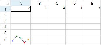
The high point is the point for the largest value. The low point is the smallest value. The negative point represents negative values. The first point is the first point that is drawn on the graph. The last point is the last point that is drawn on the graph.
The SeriesColor property applies to the line for the line spark type. The MarkersColor property is only for the line type sparkline. See the ExcelSparklineSetting class for a list of sparkline properties and additional code samples.
Using Code
- Specify a cell to create the sparkline in.
- Specify a range of cells for the data.
- Set any properties for the sparkline (such as ShowFirst and FirstMarkerColor).
- Add the sparkline to the cell.
Example
This example creates a line sparkline in a cell and shows different markers and colors.
| C# |
Copy Code
|
|---|---|
FarPoint.Win.Spread.SheetView sv = new FarPoint.Win.Spread.SheetView(); FarPoint.Win.Spread.Chart.SheetCellRange data = new FarPoint.Win.Spread.Chart.SheetCellRange(sv, 0,0,1, 5); FarPoint.Win.Spread.Chart.SheetCellRange data2 = new FarPoint.Win.Spread.Chart.SheetCellRange(sv, 5,0,1,1); FarPoint.Win.Spread.ExcelSparklineSetting ex = new FarPoint.Win.Spread.ExcelSparklineSetting(); ex.AxisColor = Color.SaddleBrown; ex.ShowFirst = true; ex.ShowHigh = true; ex.ShowLow = true; ex.ShowLast = true; ex.FirstMarkerColor = Color.Blue; ex.HighMarkerColor = Color.DarkGreen; ex.MarkersColor = Color.Aquamarine; ex.LowMarkerColor = Color.Red; ex.LastMarkerColor = Color.Orange; ex.ShowMarkers = true; fpSpread1.Sheets[0] = sv; sv.Cells[0, 0].Value = 2; sv.Cells[0, 1].Value = 5; sv.Cells[0, 2].Value = 4; sv.Cells[0, 3].Value = 1; sv.Cells[0, 4].Value = 3; fpSpread1.Sheets[0].AddSparkline(data, data2, FarPoint.Win.Spread.SparklineType.Line, ex); |
|
| VB |
Copy Code
|
|---|---|
Dim sv As New FarPoint.Win.Spread.SheetView() Dim data As New FarPoint.Win.Spread.Chart.SheetCellRange(sv, 0, 0, 1, 5) Dim data2 As New FarPoint.Win.Spread.Chart.SheetCellRange(sv, 5, 0, 1, 1) Dim ex As New FarPoint.Win.Spread.ExcelSparklineSetting() ex.AxisColor = Color.SaddleBrown ex.ShowFirst = True ex.ShowHigh = True ex.ShowLow = True ex.ShowLast = True ex.FirstMarkerColor = Color.Blue ex.HighMarkerColor = Color.DarkGreen ex.MarkersColor = Color.Aquamarine ex.LowMarkerColor = Color.Red ex.LastMarkerColor = Color.Orange ex.ShowMarkers = True fpSpread1.Sheets(0) = sv sv.Cells(0, 0).Value = 2 sv.Cells(0, 1).Value = 5 sv.Cells(0, 2).Value = 4 sv.Cells(0, 3).Value = 1 sv.Cells(0, 4).Value = 3 fpSpread1.Sheets(0).AddSparkline(data, data2, FarPoint.Win.Spread.SparklineType.Line, ex) |
|
Using the Spread Designer
- Type data in a cell or a column or row of cells in the designer.
- Select a cell for the sparkline.
- Select the Insert menu.
- Select a sparkline type.
- Select the data for the graph when the Create Sparklines dialog is displayed.
- Select OK.
- Select the sparkline cell, select the Marker Color or Sparkline Color icon, and set the colors.
- Select Apply and Exit from the File menu to save your changes and close the designer.