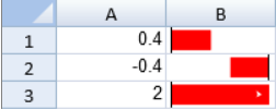
You can create an hbar sparkline using the HBARSPARKLINE formula and cell values.

The sparkline starts at the left of the cell for positive values and right of the cell for negative values. If the value is greater than 100% or smaller than -100%, an arrow is displayed.
The hbar sparkline has the following options:
| Option | Description |
| value | A number or reference that represents the length of the bar. The value should be between 100% and -100%. |
| colorScheme | A string that represents the color of the bar. This setting is optional. The default value is "grey". |
The hbar sparkline formula has the following format:
=HBARSPARKLINE(value, colorScheme)
Using Code
The following code creates hbar sparklines.
| JavaScript |
Copy Code
|
|---|---|
| activeSheet.setValue(0, 0, .4); activeSheet.setValue(1, 0, -.4); activeSheet.setValue(2, 0, 2); activeSheet.setFormula(0, 1, '=HBARSPARKLINE(A1,"red")'); activeSheet.setFormula(1, 1, '=HBARSPARKLINE(A2,"red")'); activeSheet.setFormula(2, 1, '=HBARSPARKLINE(A3,"red")'); activeSheet.setColumnWidth(0, 80); activeSheet.setColumnWidth(1, 80); |
|
See Also