You can create a Spread sparkline using the SpreadSparkline formula and cell values.
The Spread sparkline formula has the following options:
| Option | Description |
| Points | A reference that represents a range of cells that contains the values, such as "A1:A10". |
| ShowAverage | A boolean that represents whether to show the average. This setting is optional. The default value is false. |
| ScaleStart | A number that represents the minimum boundary of the sparkline. This setting is optional. The default value is the minimum of all values. |
| ScaleEnd | A number that represents the maximum boundary of the sparkline. This setting is optional. The default value is the maximum of all values. |
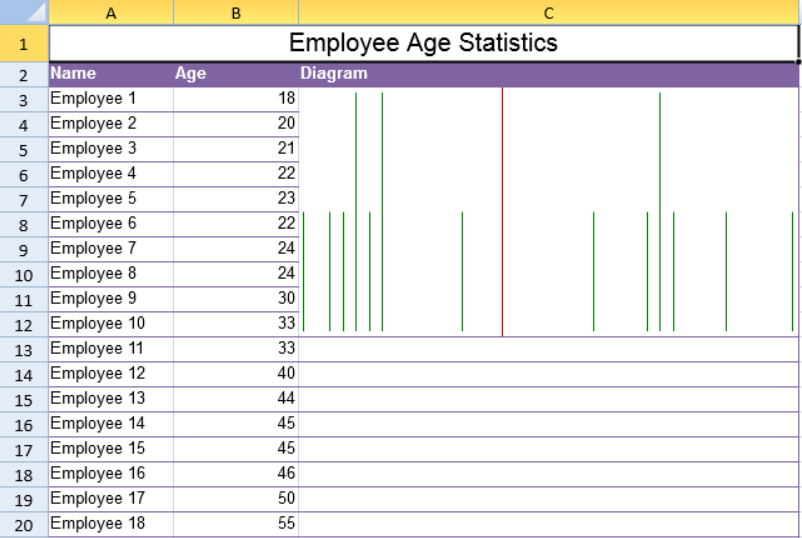
| Style | A number that references the style of the Spread sparkline. This setting is optional. The default value is 4 (poles). |
| ColorScheme | A string that represents the color of the sparkline. This setting is optional. The default value is "#646464". |
| Vertical | A boolean that represents whether to display the sparkline vertically. This setting is optional. The default value is false. |
When the sparkline is horizontal, the horizontal axis represents each point. The length of lines or the number of dots in the vertical axis represents the frequency of occurrence.
Six styles are supported:
- Stacked = 1 - line from center to two sides
- Spread = 2 - dot from center to two sides
- Jitter = 3 - dot with a random location
- Poles = 4 - line from one side to another
- StackedDots = 5 - dot from one side to another
- Stripe = 6 - line with an equal length
The Spread sparkline formula has the following format:
=SPREADSPARKLINE(points, showAverage?, scaleStart?, scaleEnd?, style?, colorScheme?, vertical?)
Using Code
The following code creates a Spread sparkline.
| JavaScript |
Copy Code
|
|---|---|
| activeSheet.addSpan(0, 0, 1, 3); activeSheet.getCell(0, 0, GC.Spread.Sheets.SheetArea.viewport).value("Employee Age Statistics").font("20px Arial").hAlign(GC.Spread.Sheets.HorizontalAlign.center).vAlign(GC.Spread.Sheets.VerticalAlign.center); var table1 = activeSheet.tables.add("table1", 1, 0, 49, 3, GC.Spread.Sheets.Tables.TableThemes.light12); table1.filterButtonVisible(false); activeSheet.setValue(1, 0, "Name"); activeSheet.setValue(1, 1, "Age"); activeSheet.setValue(1, 2, "Diagram"); for(var i = 2;i < 20; i++) { activeSheet.setValue(i, 0, "Employee " + (i - 1)); } activeSheet.setValue(2, 1, 18); activeSheet.setValue(3, 1, 20); activeSheet.setValue(4, 1, 21); activeSheet.setValue(5, 1, 22); activeSheet.setValue(6, 1, 23); activeSheet.setValue(7, 1, 22); activeSheet.setValue(8, 1, 24); activeSheet.setValue(9, 1, 24); activeSheet.setValue(10, 1, 30); activeSheet.setValue(11, 1, 33); activeSheet.setValue(12, 1, 33); activeSheet.setValue(13, 1, 40); activeSheet.setValue(14, 1, 44); activeSheet.setValue(15, 1, 45); activeSheet.setValue(16, 1, 45); activeSheet.setValue(17, 1, 46); activeSheet.setValue(18, 1, 50); activeSheet.setValue(19, 1, 55); activeSheet.addSpan(2, 2, 10, 1); activeSheet.setFormula(2, 2, '=SPREADSPARKLINE(B3:B20,TRUE,,,4,"green")'); activeSheet.setRowHeight(0, 30); activeSheet.setColumnWidth(0, 100); activeSheet.setColumnWidth(1, 100); activeSheet.setColumnWidth(2, 400); |
|
See Also