You can create a pie sparkline using the PieSparkline formula and cell values.
A cell value, cell range, or percent value can be used as percent values for the chart. The pie sparkline formula has percent and color options.
The pie formula has the following format:
=PIESPARKLINE(Percentage,color1,color2,.....)
If the percentage is a range (such as "A1:B3"), the percentage is the result of each cell's value divided by the sum of the range.
If the color parameter count is greater than or equal to the range count, values and colors have a one-to-to correspondence; redundant colors will be ignored. If the color parameter count is less than the range count, the given colors are reused and a linear gradient is used to ensure each section has a different color.
Using Code
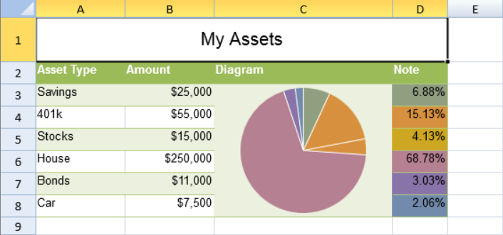
This example creates a pie sparkline.
| JavaScript |
Copy Code
|
|---|---|
| activeSheet.addSpan(0, 0, 1, 4); activeSheet.getCell(0, 0, GC.Spread.Sheets.SheetArea.viewport).value("My Assets").font("20px Arial").hAlign(GC.Spread.Sheets.HorizontalAlign.center).vAlign(GC.Spread.Sheets.VerticalAlign.center); var table1 = activeSheet.tables.add("table1", 1, 0, 7, 4, GC.Spread.Sheets.Tables.TableThemes.medium4); table1.filterButtonVisible(false); activeSheet.setValue(1, 0, "Asset Type"); activeSheet.setValue(1, 1, "Amount"); activeSheet.setValue(1, 2, "Diagram"); activeSheet.setValue(1, 3, "Note"); activeSheet.setValue(2, 0, "Savings"); activeSheet.setValue(2, 1, 25000); activeSheet.setValue(3, 0, "401k"); activeSheet.setValue(3, 1, 55000); activeSheet.setValue(4, 0, "Stocks"); activeSheet.setValue(4, 1, 15000); activeSheet.setValue(5, 0, "House"); activeSheet.setValue(5, 1, 250000); activeSheet.setValue(6, 0, "Bonds"); activeSheet.setValue(6, 1, 11000); activeSheet.setValue(7, 0, "Car"); activeSheet.setValue(7, 1, 7500); activeSheet.getRange(-1, 1, -1, 1).formatter("$#,##0"); activeSheet.addSpan(2, 2, 6, 1); activeSheet.setFormula(2, 2, '=PIESPARKLINE(B3:B8,"#919F81","#D7913E","CEA722","#B58091","#8974A9","#728BAD")'); activeSheet.getCell(2, 3, GC.Spread.Sheets.SheetArea.viewport).backColor("#919F81").formula("=B3/SUM(B3:B8)"); activeSheet.getCell(3, 3, GC.Spread.Sheets.SheetArea.viewport).backColor("#D7913E").formula("=B4/SUM(B3:B8)"); activeSheet.getCell(4, 3, GC.Spread.Sheets.SheetArea.viewport).backColor("#CEA722").formula("=B5/SUM(B3:B8)"); activeSheet.getCell(5, 3, GC.Spread.Sheets.SheetArea.viewport).backColor("#B58091").formula("=B6/SUM(B3:B8)"); activeSheet.getCell(6, 3, GC.Spread.Sheets.SheetArea.viewport).backColor("#8974A9").formula("=B7/SUM(B3:B8)"); activeSheet.getCell(7, 3, GC.Spread.Sheets.SheetArea.viewport).backColor("#728BAD").formula("=B8/SUM(B3:B8)"); activeSheet.getCell(-1, 3).formatter("0.00%"); activeSheet.setRowHeight(0, 50); for (var i = 1; i < 8; i++) { activeSheet.setRowHeight(i, 25); } activeSheet.setColumnWidth(0, 100); activeSheet.setColumnWidth(1, 100); activeSheet.setColumnWidth(2, 200); |
|
Using Code
This example creates a pie sparkline.
| JavaScript |
Copy Code
|
|---|---|
| activeSheet.addSpan(1, 0, 2, 1); activeSheet.setValue(0, 0, 40); activeSheet.setValue(0, 1, 60); activeSheet.setFormula(1, 0, '=PIESPARKLINE(A1:B1,"red","green")'); |
|